Invariant Manifold Tubes

* Türkçesi için …

As it is mentioned in the section; all asymptotic orbits, which are asymptotic to the Periodic orbits around L1 or L2, form a tube which is called invariant manifold tubes (IMT), can present lots of advantageous of mission design, esspecially they are main stuff for Low-Energy Transfers. In fact, IMT (so asymptotic orbits) is a boundary that separates the transit and non-transit tubes. As you may easily guess, transit orbits are always in IMT and can pass to one region to another. But the non-transit orbits are outside of the IMT and they are always prison in one region.

But there is a tricky thing about IMT in CR3BP. IMT are depending on periodic orbits around equilibrium points, and they can be computed thanks to them. But there are various Periodic and quasi periodic around there, so which one we should use for the IMT ? While in 2D space, there is only one periodic orbit (Horizotal Lypunov Orbit) around unstable equilibrium point in each specific energy. So that Asymptotic orbits and so IMT must be related with this periodic orbit. But in 3-dimensional space, there are more than one periodic orbits (Halo, Quasi Halo, Lissajous Orbit and Vertical Lypunov Orbit) in each specific energy, and all these periodic and quasi-periodic orbits have their own asymptotic orbits and so IMT. But in practially, 3D-IMT is generally computed with short term periodic orbits (such as vetical lyapunov or Halo orbits). In addition note that, a transit orbits seems out side of a manifold tubes while in 3-D space, this means that this transit orbits actually in another IMT of another periodic orbits.

Numeric Computation of Invariant Manifold Tubes (IMT);

As it is explained above, while computing the IMTs, Horizotal Lypunov Orbit (or some times called 2D Halo orbit) and 3D-Halo is mostly used for plotting the 2D-IMT and 3D-IMT, respectivly. First of all trajectory data of Halo orbits (H) must be found using, such as, differantial corrector method, or just try-error method for 2D-Halo orbits. Then, simply disturbing the all trajectory data of periodic orbits (H), initial condition of asymptotic orbits (X0) can be gotten easily;

X0=H±ε

H=[x, y, z, Vx, Vy, Vz] is the initial condition of Halo orbit and ε is a small (tiny) displacement from H. For 2D-IMT, the z component is neglected, of course. …. But for more simplicity and practical, the disturbance (ε) can be made only on X components. Also, (±) in equation determine the direction of IMT, which can be towards, M1, M2 or outer regions.. With to gether H and ε, the initial condition of a manifold, X0 , can be obtained simply. And also;

• if these initial conditions are integrated in forward time, unstable IMT (Departing from Halo Orbit) is gotten,
• if they are integrated in backward time, stable IMT (Approaching to Halo Orbit ) is gotten.

You can also see the matlab code of IMT in order to understand well, see bottom….. Well, now, let’s cheer up our eyes with these various IMT plots ^_^

The upper-below plots are shown IMT’s of Earth-Moon Sytem. Green ones are stable IMT, and Red ones are unstable ones.

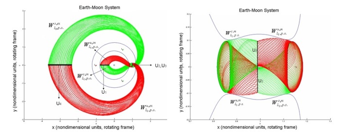
In upper, we see the 2D invariant manifold tubes of Earh Moon binary system. The notation system is borrowed from [W.S. Koon, M.W. Lo, J.E. Marsden and S.D. Ross]. The red tubes are unstable and green one are stable IMT. Also U1, U2, U3 and U4 are the section, which can be ideal for Poincare Map that it provide initial condition to jump one IMT to another; so Low energy transfers can be done.

In this upper plots, 2D-IMTs for Sun-Jupiter binary system are showed with Oterma Comet trajectory (Black trajectry). As it is seen, Oterma Comet, which is actually a transfer trajectory, is exactly in of these tubes.

In the bottom plots, 3D-IMTs for Earth-Moon binary system are showed with 3d-zero velocity surfaces. Stable and unstable tubes of inner and outer region are asigned as green and red, respectivly, while stable and unstable tubes of neck region (around Moon) are asigned as blue and pink, respectivly.

Also Let see them on work, too !

The Matlab Code of Earth-Moon’s 3D-IMTs, which give upper plot ♥ …… Just Copy, Paste and Run, ^_^ !

function manifolds_cr3bp
global mue ;
% writter: Asli Utku, 8D
mue=0.01215; C=3.16; bon=1-mue;
options = odeset('RelTol',1e-11,'AbsTol',1e-8);
figure
hold on
d=-2:0.03:2;
%..........Zero velocity surfaces ........
[X,Y,Z] = meshgrid(d,d,d);
 r1=((X + mue).^2+Y.^2+Z.^2).^(1/2);
 r2=((X + mue-1).^2+Y.^2+Z.^2).^(1/2);
 V=2*[(1/2)*(X.^2 + Y.^2)+(1-mue)./r1+mue./r2];
h = patch(isosurface(X,Y,Z,V,C),'FaceColor','black','EdgeColor','none');
camlight; lighting phong
alpha(0.1)
axis off
axis equal
% to focus to the neck reigon, make uncomment the below line
%zlim([-0.2 0.2]);xlim([0.7 1.3]);ylim([-0.2 0.2])
 view (3)
%----------------------------------------------------------------
% Equilibrium Points
y1=@(x)x-(1-mue)/(x+mue)^2+mue/(x-1+mue)^2;Lp1=fzero(y1,0);
y2=@(x)x-(1-mue)/(x+mue)^2-mue/(x-1+mue)^2;Lp2=fzero(y2,0);
y3=@(x)x+(1-mue)/(x+mue)^2+mue/(x-1+mue)^2;Lp3=fzero(y3,0);
Lp4x=0.5-mue; Lp4y=0.5*sqrt(3);
Lp5x=0.5-mue; Lp5y=-0.5*sqrt(3);
plot(Lp1,0,'r.')
plot(Lp2,0,'r.')
plot(Lp3,0,'r.')
plot(Lp4x,Lp4y,'g.')
plot(Lp5x,Lp5y,'g.')
plot(1-mue,0,'k.')
%--------------------------------------------------------------
% Halo around L1
x10=0.869581; x30=0; x50=-0.05;
x20=0; x40=-Velo(C,x10,x30,x50); x60=0;
[t,x]=ode45(@cr3bp_3b, [0 3], [x10 x20 x30 x40 x50 x60],options);
hx=x(:,1); hy=x(:,3); hz=x(:,5);
hvx=x(:,2); hvy=x(:,4); hvz=x(:,6);n=4;
% Halo around L2
x10=1.1173275; x30=0; x50=-0.03;
x20=0; x40=Velo(C,x10,x30,x50); x60=0;
[t,x]=ode45(@cr3bp_3b, [0 3.6], [x10 x20 x30 x40 x50 x60],options);
hx2=x(:,1); hy2=x(:,3); hz2=x(:,5);
hvx2=x(:,2); hvy2=x(:,4); hvz2=x(:,6);
%-----------L1 manifolds-----------
 % L1 unstable invariant manfold tube in side of neck region
 for i=1:53
x10=hx(n*i)+0.001; x30=hy(n*i); x50=hz(n*i);
x20=hvx(n*i); x40=hvy(n*i); x60=hvz(n*i);
[t,x]=ode45(@cr3bp_3b, [0 5], [x10 x20 x30 x40 x50 x60],options);m=length(t);
for ii=1:m
 if x(ii,1)>bon
 son=ii;
 break
 end
end
plot3(x(1:son,1),x(1:son,3),x(1:son,5),'m')
 end
% L1 stable invariant manfold tube in side of neck region
 for i=1:53
x10=hx(n*i)+0.00001; x30=hy(n*i); x50=hz(n*i);
x20=hvx(n*i); x40=hvy(n*i); x60=hvz(n*i);
[t,x]=ode45(@cr3bp_3b, [0 -5], [x10 x20 x30 x40 x50 x60],options);m=length(t);
for ii=1:m
 if x(ii,1)>bon
 son=ii;
 break
 end
end
plot3(x(1:son,1),x(1:son,3),x(1:son,5),'b')
 end
% L1 stable invariant manfold tube in side of inner region
for i=1:53
x10=hx(n*i)-0.0001; x30=hy(n*i); x50=hz(n*i);
x20=hvx(n*i); x40=hvy(n*i); x60=hvz(n*i);
[t,x]=ode45(@cr3bp_3b, [0 -6], [x10 x20 x30 x40 x50 x60 ],options);m=length(t);
for ii=1:m
 if x(ii,1)<0
 if x(ii,3)>0
 son=ii;
 break
 end
 end
end
 plot3(x(1:son,1),x(1:son,3),x(1:son,5),'g')
end
% L1 unstable invariant manfold tube in side of inner region
 for i=1:53
x10=hx(n*i)-0.002; x30=hy(n*i); x50=hz(n*i);
x20=hvx(n*i); x40=hvy(n*i); x60=hvz(n*i);
[t,x]=ode45(@cr3bp_3b, [0 6], [x10 x20 x30 x40 x50 x60],options);m=length(t);
for ii=1:m
 if x(ii,1)<0
 if x(ii,3)<0
 son=ii;
 break
 end
 end
end
 plot3(x(1:son,1),x(1:son,3),x(1:son,5),'r')
 end
%------------L2 manifolds--------------------------------------
% L2 stable invariant manfold tube in side of neck region
 for i=1:54
x10=hx2(n*i)-0.001; x30=hy2(n*i); x50=hz2(n*i);
x20=hvx2(n*i); x40=hvy2(n*i); x60=hvz2(n*i);
[t,x]=ode45(@cr3bp_3b, [0 -4], [x10 x20 x30 x40 x50 x60],options);m=length(t);
for ii=1:m
 if x(ii,1)<bon
 son=ii;
 break
 end
end
plot3(x(1:son,1),x(1:son,3),x(1:son,5),'b')
 end

 % L2 unstable invariant manfold tube in side of neck region
 for i=1:54
x10=hx2(n*i)-0.001; x30=hy2(n*i); x50=hz2(n*i);
x20=hvx2(n*i); x40=hvy2(n*i); x60=hvz2(n*i);
[t,x]=ode45(@cr3bp_3b, [0 4], [x10 x20 x30 x40 x50 x60],options);m=length(t);
for ii=1:m
 if x(ii,1)<bon
 son=ii;
 break
 end
end
plot3(x(1:son,1),x(1:son,3),x(1:son,5),'m')
 end

% L2 stable invariant manfold tube in side of outer region
 for i=1:54
x10=hx2(n*i)+0.0001; x30=hy2(n*i); x50=hz2(n*i); 
x20=hvx2(n*i); x40=hvy2(n*i); x60=hvz2(n*i);
[t,x]=ode45(@cr3bp_3b, [0 -10], [x10 x20 x30 x40 x50 x60],options);m=length(t);
for ii=1:m
 if x(ii,1)<0
 if x(ii,3)<0
 son=ii;
 break
 end
 end
end
 plot3(x(1:son,1),x(1:son,3),x(1:son,5),'g')
 end

 % L2 uninvariant manfold tube in side of outer region
 for i=1:54
x10=hx2(n*i)+0.0001; x30=hy2(n*i); x50=hz2(n*i); 
x20=hvx2(n*i); x40=hvy2(n*i); x60=hvz2(n*i);
[t,x]=ode45(@cr3bp_3b, [0 10], [x10 x20 x30 x40 x50 x60],options);m=length(t);
for ii=1:m
 if x(ii,1)<0
 if x(ii,3)>0
 son=ii;
 break
 end
 end
end
 plot3(x(1:son,1),x(1:son,3),x(1:son,5),'r')
 end
% oooooooooooooooooooooooooooooooooooooooooooooooooo
% halo orbits plot 
plot3(hx,hy,hz,'r') %L1
plot3(hx2,hy2,hz2,'r') %L2
%---------Jacobi integral--------------
function Vo=Velo(C,xi,yi,zi)
global mue ;
r10=sqrt((xi+mue).^2+yi.^2+zi.^2);r20=sqrt((xi-1+mue).^2+yi.^2+zi.^2);
OM0=0.5*(xi.^2+yi.^2)+(1-mue)/r10+mue/r20+0.5*mue*(1-mue);
Vo=sqrt(2*OM0-C);
%-----------------------------------
function dx = cr3bp_3b(t, x)
global mue ;
%CR3BP Equation of Motion
dx=zeros(6,1);
r1=sqrt((x(1)+mue)^2+x(3)^2+x(5)^2);
r2=sqrt((x(1)-1+mue)^2+x(3)^2+x(5)^2);
OMx=x(1)-(1-mue)*(x(1)+mue)/r1^3-mue*(x(1)-1+mue)/r2^3;
OMy=x(3)*(1-(1-mue)/r1^3-mue/r2^3);
OMz=-x(5)*((1-mue)/r1^3+mue/r2^3);
dx(1)=x(2);
dx(2)=2*x(4)+OMx;
dx(3)=x(4);
dx(4)=-2*x(2)+OMy;
dx(5)=x(6);
dx(6)=OMz;